🐼 Pandas Overview

🐼 Pandas Overview#

👨‍🏫 Vikesh K
📓 Lab 03

💡 “All great achievements require time” 💡

📝Lab Agenda#

Understanding Pandas 101
- Creating Pandas df
- Data manipulation
- Data cleaning
- Data Visualization

Tip

Use Ctrl + / to comment a code
Press H to see all the shortcuts

Pandas 101#

80% of the time you will be using Pandas function if you are working with Tabular data
It is a fast, powerful, flexible and easy to use open source data analysis and manipulation tool, built on top of the Python programming language.
Responsible for making python a popular choice for Data analysis

Importing Pandas#

import pandas as pd # launching the pandas and save it as pd
print(pd.__version__)

import os # operating system library 
print(os.getcwd()) # working directory 

2.2.0
C:\Users\vkoul\Desktop\DA_Training_book\pythonbook

In case your Pandas is not updated, uncomment and run the code below

# !pip install --upgrade pandas

# !pip install --trusted-host pypi.org --trusted-host pypi.python.org --trusted-host files.pythonhosted.org pandas

Creating Pandas DataFrame#

pandas_data_structure

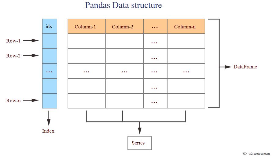
Note

Three ways to create a pandas df:

Dictionary
List
External source (csv, excel, database etc)

## From dictionary 
sample_dict = {'col_1': [3, 2, 1, 0], 'col_2': ['a', 'b', 'c', 'd']}
sample_dict

{'col_1': [3, 2, 1, 0], 'col_2': ['a', 'b', 'c', 'd']}

pd.DataFrame(sample_dict)

	col_1	col_2
0	3	a
1	2	b
2	1	c
3	0	d

## From List 
pd.DataFrame([['Imperial', 'UK'], ['Oxford', 'UK']], columns = ["University", "Country"])

	University	Country
0	Imperial	UK
1	Oxford	UK

External Source

url = 'https://raw.githubusercontent.com/vkoul/data/main/misc/titanic.csv'


df = pd.read_csv(url)
df.head(2) # show the first 2 rows of the dataset

	PassengerId	Survived	Pclass	Name	Sex	Age	SibSp	Parch	Ticket	Fare	Cabin	Embarked
0	1	0	3	Braund, Mr. Owen Harris	male	22.0	1	0	A/5 21171	7.2500	NaN	S
1	2	1	1	Cumings, Mrs. John Bradley (Florence Briggs Th...	female	38.0	1	0	PC 17599	71.2833	C85	C

Pandas Attributes and Methods#

In python, methods are functions specfic to an object type. The pandas methods allow you to do different operations on the dataset

Another aspect is attributes are like methods, but instead of transforming the variables or data they are used to give you more information about the data that you have. The attributes don’t have () at the end.

Pandas is column oriented, many of the methods are applicable at a column level

pandas_methods

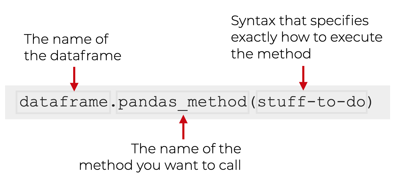
Source: J Ebener

print("There are a total of {} pandas attributes and methods".format(len(dir(pd))))

There are a total of 141 pandas attributes and methods

Useful Attributes#

Data Frame metadata

df.shape - rows and columns in the data
df.values - the values in each of the columns
df.index - this is how pandas identifies each row
df.columns - the columns in the data

Useful Methods#

DataFrame Check

df.info() - get quick info on the dataset
df.head() - check the initial 5 rows
df.tail() - check the last 5 rows
df.dtypes() - check the data types of the columns
df.sample(n) - randomly select n rows of the data

DataFrame Investigation

df.duplicated().sum() - count the duplicated values in the data
df.isna().sum() - missing values in a dataframe
df.isna().mean() - percentage of missing values in a dataframe
df.describe() - summary of the numerical columns
df.describe(include = "O") - summary of the categorical columns

Column wise analysis

df.query() - select a subset of data based on conditions
df.filter() - select only specified columns
df.assign() - add a new column to the df
df.drop() - drop columns/ rows
df.sort_values(by = "col1") - sort dataframe based on values
df.value_counts() - frequency values of a column

Summarise

df['col'].mean() - calculate the average value of the column
df['col'].median() - calculate the median value of the column
df['col'].sum() - sum up of all the values in the column
df['col'].product() - multiply all the values in the column
df['col']..agg(["mean", "median", "sum", "product"]) - agg() is very useful for doing multiple aggregations simultaneously

Other operations

df['col'].astype() - change the datatype of a column
- df['col'].astype('int') - change the datatype to integer
- df['col'].astype('object') - change the datatype to integer

📓 Case Study - Titanic#

titanic

Importing dataset#

url = 'https://raw.githubusercontent.com/vkoul/data/main/misc/titanic.csv'

# reading in the file
df = pd.read_csv(url)

Basic data investigation#

How does data look like?

type(df)

pandas.core.frame.DataFrame

df.head() # show 5 rows

	PassengerId	Survived	Pclass	Name	Sex	Age	SibSp	Ticket	Fare	Cabin	Embarked
0	1	0	3	Braund, Mr. Owen Harris	male	22.0	1	A/5 21171	7.2500	NaN	S
1	2	1	1	Cumings, Mrs. John Bradley (Florence Briggs Th...	female	38.0	1	PC 17599	71.2833	C85	C
2	3	1	3	Heikkinen, Miss. Laina	female	26.0	0	STON/O2. 3101282	7.9250	NaN	S
3	4	1	1	Futrelle, Mrs. Jacques Heath (Lily May Peel)	female	35.0	1	113803	53.1000	C123	S
4	5	0	3	Allen, Mr. William Henry	male	35.0	0	373450	8.0500	NaN	S

df.columns

Index(['PassengerId', 'Survived', 'Pclass', 'Name', 'Sex', 'Age', 'SibSp',
       'Parch', 'Ticket', 'Fare', 'Cabin', 'Embarked'],
      dtype='object')

df.index

RangeIndex(start=0, stop=891, step=1)

df.values

array([[1, 0, 3, ..., 7.25, nan, 'S'],
       [2, 1, 1, ..., 71.2833, 'C85', 'C'],
       [3, 1, 3, ..., 7.925, nan, 'S'],
       ...,
       [889, 0, 3, ..., 23.45, nan, 'S'],
       [890, 1, 1, ..., 30.0, 'C148', 'C'],
       [891, 0, 3, ..., 7.75, nan, 'Q']], dtype=object)

How many rows and columns?

df.shape

(891, 12)

Summary of the data

df.info()

<class 'pandas.core.frame.DataFrame'>
RangeIndex: 891 entries, 0 to 890
Data columns (total 12 columns):
 #   Column       Non-Null Count  Dtype  
---  ------       --------------  -----  
 0   PassengerId  891 non-null    int64  
 1   Survived     891 non-null    int64  
 2   Pclass       891 non-null    int64  
 3   Name         891 non-null    object 
 4   Sex          891 non-null    object 
 5   Age          714 non-null    float64
 6   SibSp        891 non-null    int64  
 7   Parch        891 non-null    int64  
 8   Ticket       891 non-null    object 
 9   Fare         891 non-null    float64
 10  Cabin        204 non-null    object 
 11  Embarked     889 non-null    object 
dtypes: float64(2), int64(5), object(5)
memory usage: 83.7+ KB

Column select#

How to select specific columns in the dataframe

Note

There are multiple ways of choosing a particular column in pandas

The common method is

dataframe["column_name"]

One can also use

df.column_name

If you wish to use the Pandas method

`df.filter(column_name)

In case of multiple columns:

dataframe[["col1", "col2"]]

Please select the Name column

df['Name']

                              Braund, Mr. Owen Harris
    Cumings, Mrs. John Bradley (Florence Briggs Th...
                               Heikkinen, Miss. Laina
         Futrelle, Mrs. Jacques Heath (Lily May Peel)
                             Allen, Mr. William Henry
                             ...                        
                              Montvila, Rev. Juozas
                       Graham, Miss. Margaret Edith
           Johnston, Miss. Catherine Helen "Carrie"
                              Behr, Mr. Karl Howell
                                Dooley, Mr. Patrick
Name: Name, Length: 891, dtype: object

Select only Name, Sex and Age

col_list = ['Name', 'Age', 'Sex' ]
col_list

['Name', 'Age', 'Sex']

df[col_list].head()

	Name	Age	Sex
0	Braund, Mr. Owen Harris	22.0	male
1	Cumings, Mrs. John Bradley (Florence Briggs Th...	38.0	female
2	Heikkinen, Miss. Laina	26.0	female
3	Futrelle, Mrs. Jacques Heath (Lily May Peel)	35.0	female
4	Allen, Mr. William Henry	35.0	male

OR

df.filter(col_list).head(3)

	Name	Age	Sex
0	Braund, Mr. Owen Harris	22.0	male
1	Cumings, Mrs. John Bradley (Florence Briggs Th...	38.0	female
2	Heikkinen, Miss. Laina	26.0	female

Row Filtering#

The syntax to filter rows based on a condition

df.query('column_name >= condition ') # greater than 

df.query('column_name < condition ') # less than 

df.query('column_name == "condition" ') # equal to 

Select only survived passengers

df.query('Survived == 1').head(3)

	PassengerId	Survived	Pclass	Name	Sex	Age	SibSp	Ticket	Fare	Cabin	Embarked
1	2	1	1	Cumings, Mrs. John Bradley (Florence Briggs Th...	female	38.0	1	PC 17599	71.2833	C85	C
2	3	1	3	Heikkinen, Miss. Laina	female	26.0	0	STON/O2. 3101282	7.9250	NaN	S
3	4	1	1	Futrelle, Mrs. Jacques Heath (Lily May Peel)	female	35.0	1	113803	53.1000	C123	S

df.query('Survived == 1').shape

(342, 12)

Select only female passengers

df.query("Sex == 'female'").shape

(314, 12)

df.query("Sex == 'male'").shape

(577, 12)

Mutilple Conditions

df.query('Survived == 1 & Pclass == 3').shape

(119, 12)

How many ladies survived?

df.query('Survived == 1 & Sex == "female"').shape

(233, 12)

233/314

0.7420382165605095

How many men survived?

# 💪 Please write the relevant code here
df.query('Survived == 1 & Sex == "male"').shape

(109, 12)

109/577

0.18890814558058924

Bonus question- Are the character names shown in Titanic movie real?

actors

# 💪 Please write the relevant code here

Data sorting#

Single Column sorting

df.sort_values(by = 'Age', ascending = True).head(4)

	PassengerId	Survived	Pclass	Name	Sex	Age	SibSp	Parch	Ticket	Fare	Cabin	Embarked
803	804	1	3	Thomas, Master. Assad Alexander	male	0.42	0	1	2625	8.5167	NaN	C
755	756	1	2	Hamalainen, Master. Viljo	male	0.67	1	1	250649	14.5000	NaN	S
644	645	1	3	Baclini, Miss. Eugenie	female	0.75	2	1	2666	19.2583	NaN	C
469	470	1	3	Baclini, Miss. Helene Barbara	female	0.75	2	1	2666	19.2583	NaN	C

df.sort_values(by = 'Age', ascending = False).head(3)

	PassengerId	Survived	Pclass	Name	Sex	Age	Ticket	Fare	Cabin	Embarked
630	631	1	1	Barkworth, Mr. Algernon Henry Wilson	male	80.0	27042	30.0000	A23	S
851	852	0	3	Svensson, Mr. Johan	male	74.0	347060	7.7750	NaN	S
493	494	0	1	Artagaveytia, Mr. Ramon	male	71.0	PC 17609	49.5042	NaN	C

Sort the data by Fare and check the highest price

df.sort_values(by = 'Fare', ascending = False).head(3)

	PassengerId	Survived	Pclass	Name	Sex	Age	Parch	Ticket	Fare	Cabin	Embarked
258	259	1	1	Ward, Miss. Anna	female	35.0	0	PC 17755	512.3292	NaN	C
737	738	1	1	Lesurer, Mr. Gustave J	male	35.0	0	PC 17755	512.3292	B101	C
679	680	1	1	Cardeza, Mr. Thomas Drake Martinez	male	36.0	1	PC 17755	512.3292	B51 B53 B55	C

df.sort_values(by = 'Fare', ascending = True).head(3)

	PassengerId	Survived	Pclass	Name	Sex	Age	Ticket	Cabin	Embarked
271	272	1	3	Tornquist, Mr. William Henry	male	25.0	LINE	NaN	S
597	598	0	3	Johnson, Mr. Alfred	male	49.0	LINE	NaN	S
302	303	0	3	Johnson, Mr. William Cahoone Jr	male	19.0	LINE	NaN	S

Multiple Column sorting

df.sort_values(by = ['Fare', 'Age']).head(3) # pass the column names in a list

	PassengerId	Survived	Pclass	Name	Sex	Age	Ticket	Cabin	Embarked
302	303	0	3	Johnson, Mr. William Cahoone Jr	male	19.0	LINE	NaN	S
271	272	1	3	Tornquist, Mr. William Henry	male	25.0	LINE	NaN	S
179	180	0	3	Leonard, Mr. Lionel	male	36.0	LINE	NaN	S

df.sort_values(by = ['Age', 'Fare'], ascending = [True, True]).head(3)

	PassengerId	Survived	Pclass	Name	Sex	Age	SibSp	Parch	Ticket	Fare	Cabin	Embarked
803	804	1	3	Thomas, Master. Assad Alexander	male	0.42	0	1	2625	8.5167	NaN	C
755	756	1	2	Hamalainen, Master. Viljo	male	0.67	1	1	250649	14.5000	NaN	S
469	470	1	3	Baclini, Miss. Helene Barbara	female	0.75	2	1	2666	19.2583	NaN	C

df.sort_values(by = ['Fare', 'Age'], ascending = [True, False]).head(3)

	PassengerId	Pclass	Name	Sex	Age	Ticket	Cabin	Embarked
597	598	3	Johnson, Mr. Alfred	male	49.0	LINE	NaN	S
263	264	1	Harrison, Mr. William	male	40.0	112059	B94	S
806	807	1	Andrews, Mr. Thomas Jr	male	39.0	112050	A36	S

New column creation#

df.assign(new_column = old_column and condition)

survived_mapping = {1: "Yes", 0 : "No"}
survived_mapping

{1: 'Yes', 0: 'No'}

df.assign(survived_mapped =  df['Survived'].map(survived_mapping)).head()

	PassengerId	Survived	Pclass	Name	Sex	Age	SibSp	Ticket	Fare	Cabin	Embarked	survived_mapped
0	1	0	3	Braund, Mr. Owen Harris	male	22.0	1	A/5 21171	7.2500	NaN	S	No
1	2	1	1	Cumings, Mrs. John Bradley (Florence Briggs Th...	female	38.0	1	PC 17599	71.2833	C85	C	Yes
2	3	1	3	Heikkinen, Miss. Laina	female	26.0	0	STON/O2. 3101282	7.9250	NaN	S	Yes
3	4	1	1	Futrelle, Mrs. Jacques Heath (Lily May Peel)	female	35.0	1	113803	53.1000	C123	S	Yes
4	5	0	3	Allen, Mr. William Henry	male	35.0	0	373450	8.0500	NaN	S	No

If you want to specify the location

df.insert(2, "survived_mapped", df['Survived'].map(survived_mapping))

Deleting a column

df.drop(columns = 'survived_mapped').head(3)

	PassengerId	Survived	Pclass	Name	Sex	Age	SibSp	Ticket	Fare	Cabin	Embarked
0	1	0	3	Braund, Mr. Owen Harris	male	22.0	1	A/5 21171	7.2500	NaN	S
1	2	1	1	Cumings, Mrs. John Bradley (Florence Briggs Th...	female	38.0	1	PC 17599	71.2833	C85	C
2	3	1	3	Heikkinen, Miss. Laina	female	26.0	0	STON/O2. 3101282	7.9250	NaN	S

# del df['survived_mapped']

Column rename#

df.columns

Index(['PassengerId', 'Survived', 'survived_mapped', 'Pclass', 'Name', 'Sex',
       'Age', 'SibSp', 'Parch', 'Ticket', 'Fare', 'Cabin', 'Embarked'],
      dtype='object')

Change:

Sex –> gender
survived –> survived_number

new_names = ['PassengerId', 'survived_number', 'survived_mapped', 'Pclass', 'Name', 'gender',
              'Age', 'SibSp', 'Parch', 'Ticket', 'Fare', 'Cabin_Number', 'Embarked']

print(type(new_names))

<class 'list'>

df.columns = new_names # replace the existing names with new names

df.columns

Index(['PassengerId', 'survived_number', 'survived_mapped', 'Pclass', 'Name',
       'gender', 'Age', 'SibSp', 'Parch', 'Ticket', 'Fare', 'Cabin_Number',
       'Embarked'],
      dtype='object')

You can also use the df.rename() function to change the column names

Column value replace#

Embarked location names : Southampton, Cherbourg, and Queenstown

df[['Embarked']].head(2)

	Embarked
0	S
1	C

df['Embarked'].replace({ "S": "Southampton", 
                                          "C": " Cherbourg", 
                                          "Q": "Queenstown"})

    Southampton
      Cherbourg
    Southampton
    Southampton
    Southampton
          ...     
  Southampton
  Southampton
  Southampton
    Cherbourg
   Queenstown
Name: Embarked, Length: 891, dtype: object

df['Embarked'] = df['Embarked'].replace({ "S": "Southampton", 
                                          "C": " Cherbourg", 
                                          "Q": "Queenstown"})

df[['Embarked']].head(2)

	Embarked
0	Southampton
1	Cherbourg

Data summary#

df.head(2)

	PassengerId	survived_number	survived_mapped	Pclass	Name	gender	Age	SibSp	Parch	Ticket	Fare	Cabin_Number	Embarked
0	1	0	No	3	Braund, Mr. Owen Harris	male	22.0	1	0	A/5 21171	7.2500	NaN	Southampton
1	2	1	Yes	1	Cumings, Mrs. John Bradley (Florence Briggs Th...	female	38.0	1	0	PC 17599	71.2833	C85	Cherbourg

df['Age'].mean()

29.69911764705882

Calculate avg fare

df['Fare'].mean()

32.204207968574636

df['Age'].median()

28.0

How much money titanic

df['Fare'].sum()

28693.9493

df.describe().round(3) # takes only the numerical values by default

	PassengerId	survived_number	Pclass	Age	SibSp	Parch	Fare
count	891.000	891.000	891.000	714.000	891.000	891.000	891.000
mean	446.000	0.384	2.309	29.699	0.523	0.382	32.204
std	257.354	0.487	0.836	14.526	1.103	0.806	49.693
min	1.000	0.000	1.000	0.420	0.000	0.000	0.000
25%	223.500	0.000	2.000	20.125	0.000	0.000	7.910
50%	446.000	0.000	3.000	28.000	0.000	0.000	14.454
75%	668.500	1.000	3.000	38.000	1.000	0.000	31.000
max	891.000	1.000	3.000	80.000	8.000	6.000	512.329

Details on the categorical values

df.describe(include = ['O']) # only for object

	survived_mapped	Name	gender	Ticket	Cabin_Number	Embarked
count	891	891	891	891	204	889
unique	2	891	2	681	147	3
top	No	Braund, Mr. Owen Harris	male	347082	B96 B98	Southampton
freq	549	1	577	7	4	644

Customize the percentiles

# percentiles = [0, 0.25, 0.50, 0.60, 0.75, 0.80, 0.90, 0.95, 0.99]

# df.describe(percentiles)

Summary Group wise

# df.groupby('Pclass').describe()

Exploring column data#

How many unique enteries are there?

# show the values
df['Embarked'].unique()

array(['Southampton', ' Cherbourg', 'Queenstown', nan], dtype=object)

# count the value
df['Embarked'].nunique()

What is the frequency count?

df["Embarked"].value_counts(dropna= False) # by default its true

Embarked
Southampton    644
 Cherbourg     168
Queenstown      77
NaN              2
Name: count, dtype: int64

df["Embarked"].value_counts(dropna= False, normalize = True) # by default its true

Embarked
Southampton    0.722783
 Cherbourg     0.188552
Queenstown     0.086420
NaN            0.002245
Name: proportion, dtype: float64

df["Pclass"].value_counts(dropna= False, normalize = True).round(3) 

Pclass
3    0.551
1    0.242
2    0.207
Name: proportion, dtype: float64

df["Embarked"].value_counts(dropna= False, normalize = True).round(2) # get the percenatge 

Embarked
Southampton    0.72
 Cherbourg     0.19
Queenstown     0.09
NaN            0.00
Name: proportion, dtype: float64

Data manipulation#

Tip

Useful functions are (click on the links) :

# example code
# pd.pivot_table(index = 'survived_mapped', columns = "Pclass", data = df)['Fare'].round(2)

What is the distrbution of Survived passengers across pclass

df["survived_mapped"].value_counts()

survived_mapped
No     549
Yes    342
Name: count, dtype: int64

df["survived_mapped"].value_counts(normalize = True).round(2)

survived_mapped
No     0.62
Yes    0.38
Name: proportion, dtype: float64

pd.crosstab(df["survived_mapped"], df["Pclass"])

Pclass	1	2	3
survived_mapped
No	80	97	372
Yes	136	87	119

pd.crosstab(df["survived_mapped"], df["gender"])

gender	female	male
survived_mapped
No	81	468
Yes	233	109

Grouping data#

Group by allows you to calculate numeric summaries across a categorical value

split_apply_combine

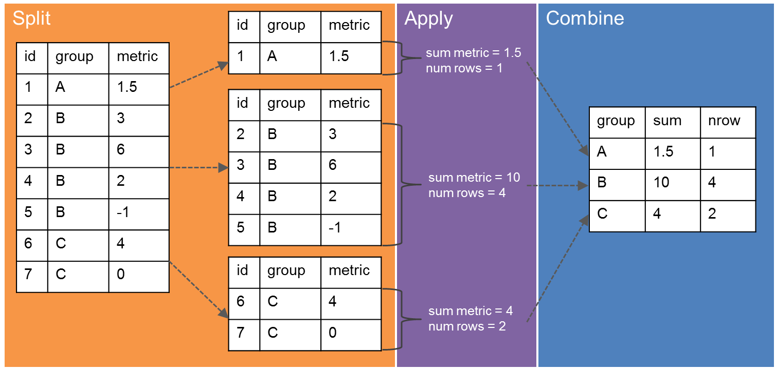
What is the average age for each gender group

# calculating the mean for the column
df["Age"].mean()

29.69911764705882

# calculating the mean based on Sex group
df.groupby("gender")["Age"].mean().round(2)

gender
female    27.92
male      30.73
Name: Age, dtype: float64

# calculating the mean based on Pclass
df.groupby("Pclass")["Age"].mean().round()

Pclass
1    38.0
2    30.0
3    25.0
Name: Age, dtype: float64

# calculating the mean based on Pclass
df.groupby("Pclass")["Fare"].mean().round()

Pclass
1    84.0
2    21.0
3    14.0
Name: Fare, dtype: float64

# calculating the mean based on Pclass
df.groupby("Pclass")["Fare"].median().round()

Pclass
1    60.0
2    14.0
3     8.0
Name: Fare, dtype: float64

df.groupby("column")["numeric_column"].whichfunction()

# calculating the mean based on Sex group
df.groupby(["Pclass", "gender"])["Age"].mean().reset_index().round(1)

	Pclass	gender	Age
0	1	female	34.6
1	1	male	41.3
2	2	female	28.7
3	2	male	30.7
4	3	female	21.8
5	3	male	26.5

# calculating the mean based on Sex group
df.groupby(["Pclass", "gender"])["Fare"].median().reset_index().round(1)

	Pclass	gender	Fare
0	1	female	82.7
1	1	male	41.3
2	2	female	22.0
3	2	male	13.0
4	3	female	12.5
5	3	male	7.9

# calculating the mean based on Sex group
df.groupby(["Pclass", "gender", "survived_mapped"])["Fare"].mean().reset_index().round(1)

	Pclass	gender	survived_mapped	Fare
0	1	female	No	110.6
1	1	female	Yes	106.0
2	1	male	No	62.9
3	1	male	Yes	74.6
4	2	female	No	18.2
5	2	female	Yes	22.3
6	2	male	No	19.5
7	2	male	Yes	21.1
8	3	female	No	19.8
9	3	female	Yes	12.5
10	3	male	No	12.2
11	3	male	Yes	15.6

# calculating the mean based on Sex group
df.groupby(["Pclass", "gender"])["Age"].mean().reset_index().round(2)

	Pclass	gender	Age
0	1	female	34.61
1	1	male	41.28
2	2	female	28.72
3	2	male	30.74
4	3	female	21.75
5	3	male	26.51

Groupby on multiple columns and aggregations on different columns

# # calculating the mean based on Sex group
df.groupby(["Pclass", "gender"]).agg({'Age':'mean', 'Fare':'median'}).round(2).reset_index()

	Pclass	gender	Age	Fare
0	1	female	34.61	82.66
1	1	male	41.28	41.26
2	2	female	28.72	22.00
3	2	male	30.74	13.00
4	3	female	21.75	12.48
5	3	male	26.51	7.92

Changing the column data type#

Often, we need to convert the datatype of a column. We will make use of the .astype() method to achieve this.

# calling a single column
df['Pclass']

    3
    1
    3
    1
    3
      ..
  2
  1
  3
  1
  3
Name: Pclass, Length: 891, dtype: int64

type(df['Pclass'])

pandas.core.series.Series

# converting the Pclass to an object from integer
df['Pclass'].astype('object')

    3
    1
    3
    1
    3
      ..
  2
  1
  3
  1
  3
Name: Pclass, Length: 891, dtype: object

# Replace the original column with the new modified column
df['Pclass'] = df['Pclass'].astype('object')

df['Pclass'] 

    3
    1
    3
    1
    3
      ..
  2
  1
  3
  1
  3
Name: Pclass, Length: 891, dtype: object

Missing values#

Note

Pandas has got extensive functions to deal with missing data

df.isna() or df.isnull()
df.notna() or df.notnull()
df.fillna()
df.dropna()

Get the sum of missing values across columns

df.isna().sum()

PassengerId          0
survived_number      0
survived_mapped      0
Pclass               0
Name                 0
gender               0
Age                177
SibSp                0
Parch                0
Ticket               0
Fare                 0
Cabin_Number       687
Embarked             2
dtype: int64

Get the sum of missing values across rows

df.isna().sum(axis = 1)

    1
    0
    1
    0
    1
      ..
  1
  0
  2
  0
  1
Length: 891, dtype: int64

# df.head()

Get the percentage of missing values across columns

df.isna().mean().round(2)

PassengerId        0.00
survived_number    0.00
survived_mapped    0.00
Pclass             0.00
Name               0.00
gender             0.00
Age                0.20
SibSp              0.00
Parch              0.00
Ticket             0.00
Fare               0.00
Cabin_Number       0.77
Embarked           0.00
dtype: float64

Adding the missing rows as a new column to the dataframe

df["missing_rows"] = df.isna().sum(axis = 1)

# check the new column at the end
df.head()

	PassengerId	survived_number	survived_mapped	Pclass	Name	gender	Age	SibSp	Ticket	Fare	Cabin_Number	Embarked	missing_rows
0	1	0	No	3	Braund, Mr. Owen Harris	male	22.0	1	A/5 21171	7.2500	NaN	Southampton	1
1	2	1	Yes	1	Cumings, Mrs. John Bradley (Florence Briggs Th...	female	38.0	1	PC 17599	71.2833	C85	Cherbourg	0
2	3	1	Yes	3	Heikkinen, Miss. Laina	female	26.0	0	STON/O2. 3101282	7.9250	NaN	Southampton	1
3	4	1	Yes	1	Futrelle, Mrs. Jacques Heath (Lily May Peel)	female	35.0	1	113803	53.1000	C123	Southampton	0
4	5	0	No	3	Allen, Mr. William Henry	male	35.0	0	373450	8.0500	NaN	Southampton	1

# subseting the data only for rows with more than 1 missing rows
df.query("missing_rows > 1").head()

	PassengerId	survived_number	survived_mapped	Pclass	Name	gender	Age	Ticket	Fare	Cabin_Number	Embarked	missing_rows
5	6	0	No	3	Moran, Mr. James	male	NaN	330877	8.4583	NaN	Queenstown	2
17	18	1	Yes	2	Williams, Mr. Charles Eugene	male	NaN	244373	13.0000	NaN	Southampton	2
19	20	1	Yes	3	Masselmani, Mrs. Fatima	female	NaN	2649	7.2250	NaN	Cherbourg	2
26	27	0	No	3	Emir, Mr. Farred Chehab	male	NaN	2631	7.2250	NaN	Cherbourg	2
28	29	1	Yes	3	O'Dwyer, Miss. Ellen "Nellie"	female	NaN	330959	7.8792	NaN	Queenstown	2

Find column which have atleast three missing values

# df.isna().sum() >= 3

Joining Data#

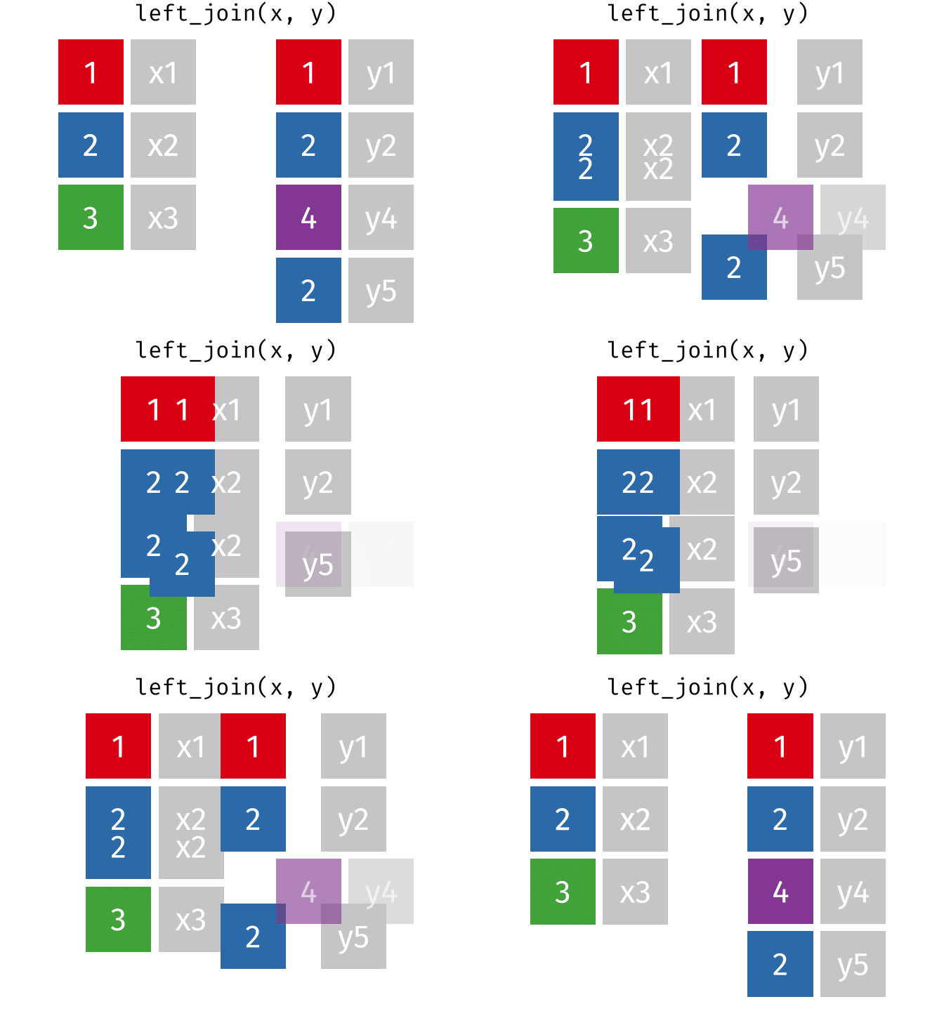
While working on a problem, you would require to join datasets from different sources. Very important to understand different joins and how to do it in python

The major joins used are: left, inner, right, cross

The below animations are from here

Left join

df1.merge(df2, on = 'column_name', how = 'left') 

left_join

Inner join

df1.merge(df2, on = 'column_name', how = 'inner') 

inner_join

Right join

df1.merge(df2, on = 'column_name', how = 'right') 

right_join

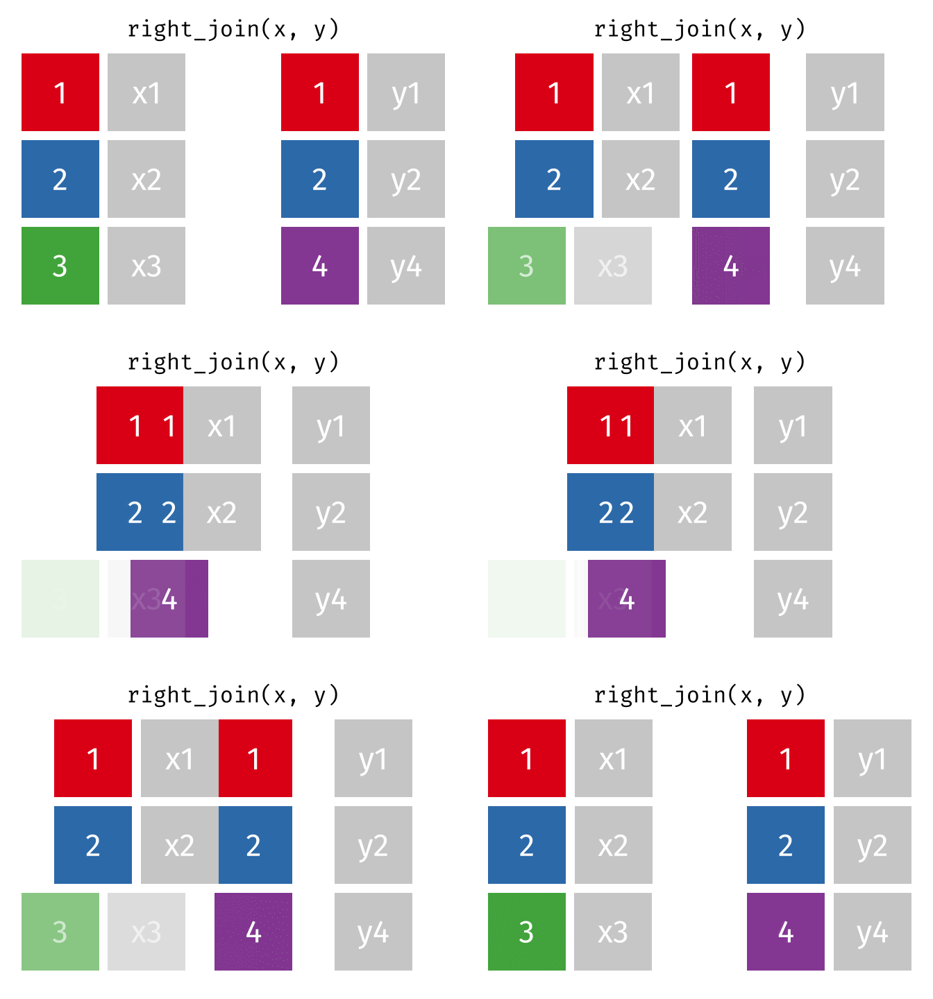
Lets create a class data-frame which we will join the to titanic dataset

class_details = pd.DataFrame({"Pclass": [1, 2, 3] , "Class": ["FirstC", "SecondC", "ThirdC"]})
class_details

	Pclass	Class
0	1	FirstC
1	2	SecondC
2	3	ThirdC

# Check the dimensions of df dataset
df.shape

(891, 14)

df.merge(class_details, on = "Pclass", how = 'left').head(2)

	PassengerId	survived_number	survived_mapped	Pclass	Name	gender	Age	SibSp	Parch	Ticket	Fare	Cabin_Number	Embarked	missing_rows	Class
0	1	0	No	3	Braund, Mr. Owen Harris	male	22.0	1	0	A/5 21171	7.2500	NaN	Southampton	1	ThirdC
1	2	1	Yes	1	Cumings, Mrs. John Bradley (Florence Briggs Th...	female	38.0	1	0	PC 17599	71.2833	C85	Cherbourg	0	FirstC

df = df.merge(class_details, on = "Pclass", how = 'left')

# Check the dimensions of df dataset
df.shape

(891, 15)

Inbuilt Plotting#

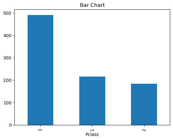
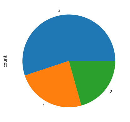
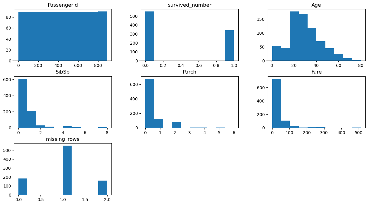
Pandas has an inbuilt method to quickly plot charts

df.hist() - for numeric values
df['column'].plot( kind = 'Chart type') - synatx for plotting

df.value_counts('Pclass')

Pclass
3    491
1    216
2    184
Name: count, dtype: int64

df['Pclass'].value_counts().plot(kind = 'bar', title = "Bar Chart");

_images/570bc7280a830409a2e9d0887b563226cfa407c91fff04358924242ec60772a4.png

df['Pclass'].value_counts().plot(kind = 'pie');

_images/c5a71d16dee62395ff576688f677c1728d5fb02fa9ff28ecda48879701b66809.png

df.hist(figsize = (15, 8), grid = False);

_images/ce84cb2c589d966f0e0515d7d5b84dc5052fa5caa30fc91fdcb197299fe9c146.png

Exporting a file#

csv format

df.to_csv("Titanic_modified_Python_processed.csv", index = False)

print("The csv file is exported to {}".format(os.getcwd()))

The csv file is exported to C:\Users\vkoul\Desktop\DA_Training_book\pythonbook

xlsx format

df.to_excel("Titanic_modified_Python_processed.xlsx", index = False)

print("The csv file is exported to {}".format(os.getcwd()))

C:\Users\vkoul\AppData\Local\Temp\1\ipykernel_25136\222098466.py:1: UserWarning: Pandas requires version '3.0.5' or newer of 'xlsxwriter' (version '3.0.3' currently installed).
  df.to_excel("Titanic_modified_Python_processed.xlsx", index = False)

The csv file is exported to C:\Users\vkoul\Desktop\DA_Training_book\pythonbook

Tip

Best Way to learn Pandas is to download datasets, prepare a list of questions and answer those questions using Pandas

Kaggle Datasets is a good website to get relevant website

📚 Reference material#

Pandas

Pandas Exercises - Highly recommend
Community tutorials - very useful
40 Examples to Master Pandas- very useful
Pandas CookBook- Good reference
Modern Pandas - Good Reference
10 mins pandas - Definitely check this out to get a quick introduction to pandas
Data Manipulation with Pandas

Pandas Documentation

🐼 Pandas Overview

Contents

🐼 Pandas Overview#

📝Lab Agenda#

Pandas 101#

Importing Pandas#

Creating Pandas DataFrame#

Pandas Attributes and Methods#

Useful Attributes#

Useful Methods#

📓 Case Study - Titanic#

Importing dataset#

Basic data investigation#

Column select#

Row Filtering#

Data sorting#

New column creation#

Column rename#

Column value replace#

Data summary#

Exploring column data#

Data manipulation#

Grouping data#

Changing the column data type#

Missing values#

Joining Data#

Inbuilt Plotting#

Exporting a file#

📚 Reference material#